ANFIS variants
Neuro-Fuzzy Toolbox provides three distinct classes for working with ANFIS models. Each of them can handle both regression and classification problems (binary and multiclass). The differences between these classes lie in the internal structure of the model and in the way its parameters are stored.
1. Classical ANFIS
The classical ANFIS model (neuro_fuzzy_toolbox.models.ANFIS) allows
a different number of membership functions (MFs) for each input feature.
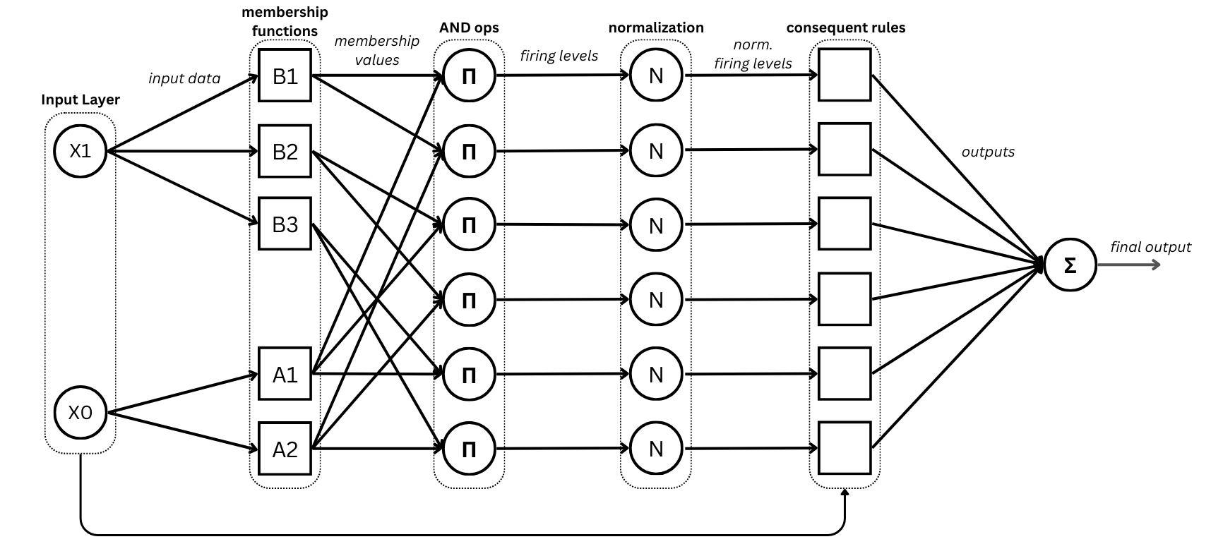
ANFIS model for 2-feature data, where the first feature has 2 membership functions and the second has 3 (source: authors).
The parameters available for instantiating an ANFIS model are the following:
mf_distribution: List containing the number of MFs for each input feature.
outputs: Number of model outputs. Default is 1.
membership_function: MF to use. Default is
GeneralizedBell_MF.output_type: Defines the output layer of the model. Accepted values are
'default'(no output layer; classical mode for regression problems),'sigmoid'(output layer with sigmoid activation), and'softmax'(output layer with softmax activation). Default is'default'.features: Iterable containing the names of the input variables as strings. Default is
None, which produces the list [x0, x1, …].dtype: Data type of the tensors holding the model parameters. Default is
torch.float32.
Note
A simple instantiation example was already shown in the previous section (ANFIS Model Basics).
2. Homogeneous ANFIS
The homogeneous ANFIS model (neuro_fuzzy_toolbox.models.h_ANFIS) is
a classical ANFIS model in which all input features share the same number of
MFs. The only difference with respect to the classical ANFIS is the way the
premise parameters are stored: in this case they are stored in a single
tensor, which improves computational efficiency.
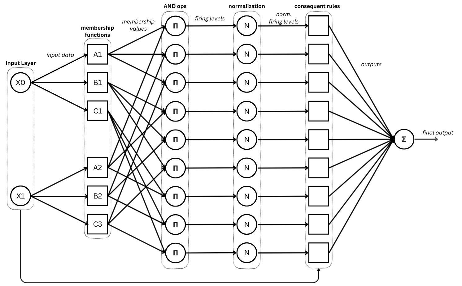
ANFIS model for 2-feature data, where both features have 3 membership functions (source: authors).
The parameters available for instantiating this class are the following:
input_size: Number of input features.
num_mfs: Number of MFs per feature.
outputs: Number of model outputs. Default is 1.
membership_function: MF to use. Default is
GeneralizedBell_MF.output_type: Defines the output layer of the model. Accepted values are
'default'(no output layer; classical mode for regression problems),'sigmoid'(output layer with sigmoid activation), and'softmax'(output layer with softmax activation). Default is'default'.rule_reduced:
Trueto instantiate a rule-reduced ANFIS model,Falseotherwise. Default isFalse.features: Iterable containing the names of the input variables as strings. Default is
None, which produces the list [x0, x1, …].dtype: Data type of the tensors holding the model parameters. Default is
torch.float32.
Unlike neuro_fuzzy_toolbox.models.ANFIS, the number of features and
the number of MFs are specified separately, since all features are assumed to
share the same number of MFs.
Important
The rule_reduced parameter allows a rule-reduced ANFIS model to be instantiated (see rule-reduced ANFIS).
The key difference between both classes lies in the way the premise parameters are stored.
Class |
Premise structure |
|---|---|
ANFIS |
List of 2D tensors of shape \((num\_mfs \times num\_params)\) |
h_ANFIS |
Single 3D tensor of shape \((input\_size \times num\_mfs \times num\_params)\) |
Note
More specifically, the premises in neuro_fuzzy_toolbox.models.ANFIS
are stored in an nn.ParameterList — a list of nn.Parameter objects,
each associated with a specific input feature and holding a 2D tensor with
the MF parameters for that feature (see the official documentation:
nn.Parameter
and
nn.ParameterList).
In neuro_fuzzy_toolbox.models.h_ANFIS, the premises are stored in
a single nn.Parameter holding a 3D tensor with all premise parameters,
which is what makes the operations computationally more efficient.
Example
The following example considers an ANFIS model for 4-feature data, where all features have 3 MFs:
# Simulating a dataset of 200 samples with 4 features
x_train = 2 * torch.rand(200, 4) - 1  # shape must be (200, 4)
Both classes are instantiated for comparison:
anfis_model = nft.ANFIS(
    mf_distribution=[3, 3, 3, 3],  # MF distribution across features
    membership_function=nft.Gaussian_MF
)

h_anfis = nft.h_ANFIS(
    input_size=x_train.shape[1],
    num_mfs=3,                      # same number of MFs per feature
    membership_function=nft.Gaussian_MF
)

# Initialize premises of both models with the same values for comparison
anfis_model.init_premises(x_train)
h_anfis.init_premises(x_train)
ANFIS (list structure)
anfis_model.get_premises() # Output: list of tensors (one per feature) of shape (mfs × params)
[tensor([[-0.9999,  0.4968],
         [-0.0062,  0.4968],
         [ 0.9874,  0.4968]]),
 tensor([[-0.9844,  0.4941],
         [ 0.0039,  0.4941],
         [ 0.9921,  0.4941]]),
 tensor([[-9.9330e-01,  4.9635e-01],
         [-6.0350e-04,  4.9635e-01],
         [ 9.9209e-01,  4.9635e-01]]),
 tensor([[-9.9768e-01,  4.9846e-01],
         [-7.5603e-04,  4.9846e-01],
         [ 9.9617e-01,  4.9846e-01]])]
This method is designed to facilitate visualization and manipulation of the
premise parameters. Internally, however, the premises are stored in an
nn.ParameterList where each element holds a 2D tensor of shape
\((num\_mfs \times num\_params)\) corresponding to a specific input
feature.
Using the get_premises_as_parameters_list() method returns:
anfis_model.get_premises_as_parameters_list()
ParameterList(
    (0): Parameter containing: [torch.float32 of size 3x2]
    (1): Parameter containing: [torch.float32 of size 3x2]
    (2): Parameter containing: [torch.float32 of size 3x2]
    (3): Parameter containing: [torch.float32 of size 3x2]
)
h_ANFIS (3D tensor structure)
h_anfis.get_premises() # Output: unified 3D tensor of shape (features × mfs × params)
tensor([[[-9.9992e-01,  4.9684e-01],
         [-6.2422e-03,  4.9684e-01],
         [ 9.8744e-01,  4.9684e-01]],

        [[-9.8438e-01,  4.9413e-01],
         [ 3.8766e-03,  4.9413e-01],
         [ 9.9214e-01,  4.9413e-01]],

        [[-9.9330e-01,  4.9635e-01],
         [-6.0350e-04,  4.9635e-01],
         [ 9.9209e-01,  4.9635e-01]],

        [[-9.9768e-01,  4.9846e-01],
         [-7.5603e-04,  4.9846e-01],
         [ 9.9617e-01,  4.9846e-01]]])
Using the get_premises_as_parameters_list() method returns:
h_anfis.get_premises_as_parameters_list()
[Parameter containing:
 tensor([[[-9.9992e-01,  4.9684e-01],
          [-6.2422e-03,  4.9684e-01],
          [ 9.8744e-01,  4.9684e-01]],

         [[-9.8438e-01,  4.9413e-01],
          [ 3.8766e-03,  4.9413e-01],
          [ 9.9214e-01,  4.9413e-01]],

         [[-9.9330e-01,  4.9635e-01],
          [-6.0350e-04,  4.9635e-01],
          [ 9.9209e-01,  4.9635e-01]],

         [[-9.9768e-01,  4.9846e-01],
          [-7.5603e-04,  4.9846e-01],
          [ 9.9617e-01,  4.9846e-01]]], requires_grad=True)]
3. Rule-reduced ANFIS
The rule-reduced ANFIS model is a variant of the homogeneous ANFIS that reduces the number of rules by associating each MF with a single input feature. This means that each rule in the model is fully independent of the others, since the combinatorial rule construction of the classical model across MFs is not performed.
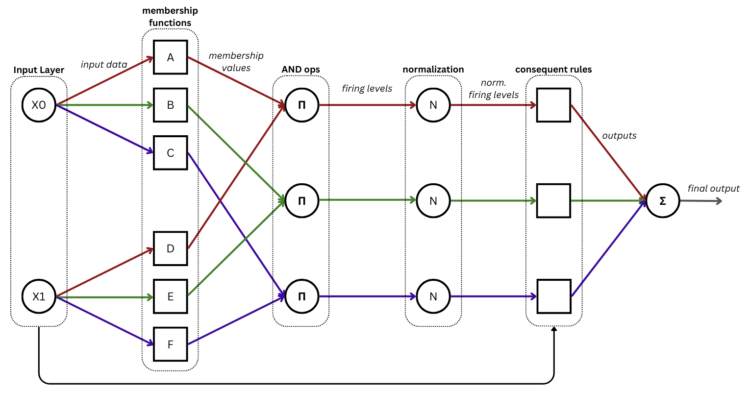
Rule-reduced ANFIS model for 2-feature data, where both features have 3 membership functions (source: authors).
This ANFIS variant is particularly useful when working with high-dimensional datasets, since the number of rules and consequent parameters is considerably reduced, enabling more efficient training.
The rule generation process is illustrated in the following comparison figure:
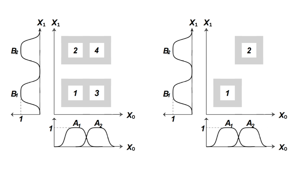
Comparison between rule generation in a classical ANFIS model (left) and a rule-reduced ANFIS model (right) for 2-feature data, where both have 2 MFs per feature. In the classical model, rules are generated using all combinations of MFs; in the rule-reduced model, each MF in a feature is associated with a single rule together with exactly one MF from each of the remaining features (source: authors).
This model can be instantiated in two ways: using the dedicated
neuro_fuzzy_toolbox.models.rule_reduced_ANFIS class (see
rule-reduced ANFIS class), or using
neuro_fuzzy_toolbox.models.h_ANFIS with the additional parameter
rule_reduced=True.
3.1 Rule-reduced h_ANFIS
As mentioned above, the rule-reduced ANFIS model can be instantiated using
neuro_fuzzy_toolbox.models.h_ANFIS with rule_reduced=True:
# Simulating a dataset of 200 samples with 3 features
x_train = 2 * torch.rand(200, 3) - 1  # shape must be (200, 3)

rule_reduced_anfis = nft.h_ANFIS(
    input_size=x_train.shape[1],  # number of features, in this case 3
    num_mfs=3,                    # same number of MFs per feature
    membership_function=nft.GeneralizedBell_MF,
    rule_reduced=True             # enables rule-reduced mode
)
Tip
This variant is the most computationally efficient, as it leverages the
internal structure of the h_ANFIS class: premises and consequents are
each stored in a single 3D tensor of shape
\((input\_size \times num\_mfs \times num\_params)\) and
\((outputs \times rules \times (input\_size + 1))\) respectively, and
the number of generated rules is reduced. The dedicated
rule-reduced ANFIS class stores
parameters differently, which has other advantages.
3.2 Rule-reduced ANFIS class
neuro_fuzzy_toolbox.models.rule_reduced_ANFIS is a dedicated class
for working with rule-reduced ANFIS models. In this class, both premise and
consequent parameters are stored differently from the other model classes.
The instantiation parameters are the same as those of the homogeneous ANFIS model (homogeneous ANFIS), with one additional parameter:
input_size: Number of input features.
num_mfs: Number of MFs per feature.
outputs: Number of model outputs. Default is 1.
membership_function: MF to use. Default is
GeneralizedBell_MF.output_type: Defines the output layer of the model. Accepted values are
'default'(no output layer; classical mode for regression problems),'sigmoid'(output layer with sigmoid activation), and'softmax'(output layer with softmax activation). Default is'default'.default_rule (
EXPERIMENTAL):Trueto include a default rule,Falseotherwise. Default isFalse.features: Iterable containing the names of the input variables as strings. Default is
None, which produces the list [x0, x1, …].dtype: Data type of the tensors holding the model parameters. Default is
torch.float32.
Caution
The default_rule parameter is under active development. Its behavior
may change and some functionalities may not yet be available. It adds an
extra firing level to capture all input combinations not covered by the
model’s reduced rule set.
The key difference between this class and
neuro_fuzzy_toolbox.models.h_ANFIS with rule_reduced=True lies
in how the premise and consequent parameters are stored:
The premises are stored in an
nn.ParameterListwhere each element contains the MFs associated with a single rule of the model — that is, a 2D tensor of shape \((input\_size \times num\_params)\), where \(num\_params\) is the number of parameters of the chosen MF.The consequents are also stored in an
nn.ParameterList, where each element contains the consequent parameters associated with a single rule — that is, a 2D tensor of shape \((outputs \times (input\_size + 1))\).
Although the internal storage differs from the h_ANFIS class, the API is
the same. The following example instantiates two rule-reduced ANFIS models
(one with each class) to illustrate their differences.
# Simulating a dataset of 200 samples with 4 features
x_train = 2 * torch.rand(200, 4) - 1  # shape must be (200, 4)

h_anfis_rule_reduced = nft.h_ANFIS(
    input_size=x_train.shape[1],  # number of features, in this case 4
    num_mfs=3,                    # same number of MFs per feature
    membership_function=nft.Gaussian_MF,
    rule_reduced=True
)

rule_reduced_anfis = nft.rule_reduced_ANFIS(
    input_size=x_train.shape[1],  # number of features, in this case 4
    num_mfs=3,                    # same number of MFs per feature
    membership_function=nft.Gaussian_MF
)

# Set both models to the same parameter values for comparison
h_anfis_rule_reduced.set_premises(rule_reduced_anfis.get_premises())
h_anfis_rule_reduced.set_consequents(rule_reduced_anfis.get_consequents())
Premises
h_anfis_rule_reduced.get_premises()

rule_reduced_anfis.get_premises()
Both return a 3D tensor of shape
\((input\_size \times num\_mfs \times num\_params)\), where
\(num\_params\) is the number of parameters of the chosen MF (in this
case Gaussian_MF with parameters \(\mu\) and \(\sigma\)).
tensor([[[ 0.0075,  0.9413],
         [-0.9569,  0.1347],
         [-0.8626,  0.9480]],

        [[-0.7637,  0.3460],
         [-0.5524,  0.1475],
         [ 0.1900,  0.3439]],

        [[ 0.8265,  0.4483],
         [ 0.5921,  0.9003],
         [-0.9505,  0.8001]],

        [[ 0.0264,  1.0643],
         [ 0.3168,  0.6440],
         [-0.4060,  0.5463]]])
However, calling get_premises_as_parameters_list() returns different structures for each class:
h_anfis_rule_reduced instance
h_anfis_rule_reduced.get_premises_as_parameters_list()
[Parameter containing:
 tensor([[[ 0.0075,  0.9413],
          [-0.9569,  0.1347],
          [-0.8626,  0.9480]],

         [[-0.7637,  0.3460],
          [-0.5524,  0.1475],
          [ 0.1900,  0.3439]],

         [[ 0.8265,  0.4483],
          [ 0.5921,  0.9003],
          [-0.9505,  0.8001]],

         [[ 0.0264,  1.0643],
          [ 0.3168,  0.6440],
          [-0.4060,  0.5463]]], requires_grad=True)]
rule_reduced_ANFIS instance
rule_reduced_anfis.get_premises_as_parameters_list()
ParameterList(
    (0): Parameter containing: [torch.float32 of size 4x2]
    (1): Parameter containing: [torch.float32 of size 4x2]
    (2): Parameter containing: [torch.float32 of size 4x2]
)
To inspect the values of each element:
for i, rule in enumerate(rule_reduced_anfis.get_premises_as_parameters_list()):
    print(f"Rule {i+1} premises:\n", rule, "\n")
Rule 1 premises:
 Parameter containing:
tensor([[ 0.0075,  0.9413],
        [-0.7637,  0.3460],
        [ 0.8265,  0.4483],
        [ 0.0264,  1.0643]], requires_grad=True)

Rule 2 premises:
 Parameter containing:
tensor([[-0.9569,  0.1347],
        [-0.5524,  0.1475],
        [ 0.5921,  0.9003],
        [ 0.3168,  0.6440]], requires_grad=True)

Rule 3 premises:
 Parameter containing:
tensor([[-0.8626,  0.9480],
        [ 0.1900,  0.3439],
        [-0.9505,  0.8001],
        [-0.4060,  0.5463]], requires_grad=True)
As noted above, each tensor has shape \((input\_size \times num\_params)\),
where \(num\_params\) is the number of parameters of the chosen MF. In
this case Gaussian_MF uses parameters \([\mu, \sigma]\), and each
set of \(input\_size\) pairs (4 in this example) is combined to form one
rule, giving a total of 3 rules.
Tip
The get_premises_as_parameters_list() method is useful for initializing PyTorch optimizers when implementing custom training procedures. See Custom training for details.
Consequents
The same pattern applies to the consequent parameters:
h_anfis_rule_reduced.get_consequents()

rule_reduced_anfis.get_consequents()
Both return a 3D tensor of shape \((outputs \times rules \times (input\_size + 1))\), where the \(+1\) corresponds to the bias term.
tensor([[[-0.0272,  0.0149, -0.0077,  0.4051,  0.4818],
         [ 0.7763, -0.9301,  0.4228,  0.0454, -0.3164],
         [ 0.8950, -0.8065, -0.5194,  0.7518, -0.2449]]])
Note
The classical ANFIS model generates rules using all possible combinations of MFs, so the number of rules would be \(num\_mfs^{input\_size}\) (in this case \(3^4 = 81\)), with each rule having \(input\_size + 1\) consequent parameters (5 in this case, including the bias). In the rule-reduced model, however, rules are not generated combinatorially: each MF in a given feature is associated with a single rule, together with exactly one MF from each of the remaining features. This means the number of rules equals the number of MFs per feature, which is 3 in this case (see the comparison figure for a visual illustration of the difference).
Calling get_consequents_as_parameters_list() again returns different structures for each class:
h_anfis_rule_reduced instance
h_anfis_rule_reduced.get_consequents_as_parameters_list()
[Parameter containing:
 tensor([[[-0.0272,  0.0149, -0.0077,  0.4051,  0.4818],
          [ 0.7763, -0.9301,  0.4228,  0.0454, -0.3164],
          [ 0.8950, -0.8065, -0.5194,  0.7518, -0.2449]]], requires_grad=True)]
rule_reduced_ANFIS instance
rule_reduced_anfis.get_consequents_as_parameters_list()
ParameterList(
    (0): Parameter containing: [torch.float32 of size 1x5]
    (1): Parameter containing: [torch.float32 of size 1x5]
    (2): Parameter containing: [torch.float32 of size 1x5]
)
To inspect the values of each element:
for i, rule in enumerate(rule_reduced_anfis.get_consequents_as_parameters_list()):
    print(f"Rule {i+1} consequents:\n", rule, "\n")
Rule 1 consequents:
 Parameter containing:
tensor([[-0.0272,  0.0149, -0.0077,  0.4051,  0.4818]], requires_grad=True)

Rule 2 consequents:
 Parameter containing:
tensor([[ 0.7763, -0.9301,  0.4228,  0.0454, -0.3164]], requires_grad=True)

Rule 3 consequents:
 Parameter containing:
tensor([[ 0.8950, -0.8065, -0.5194,  0.7518, -0.2449]], requires_grad=True)
Each tensor has shape \((outputs \times (input\_size + 1))\), where the \(+1\) corresponds to the bias term. In other words, each tensor holds the consequent parameters associated with a single rule (for each model output; 1 in this case).
Rules-based storage structure
As described above, neuro_fuzzy_toolbox.models.rule_reduced_ANFIS
stores premises and consequents in parameter lists where each element is
associated with a specific rule. This design is intended to facilitate
manipulation of the model’s rule structure.
Note
This is leveraged by the SONFIS algorithm, and may also be useful for Custom Training.