ANFIS Model Basics

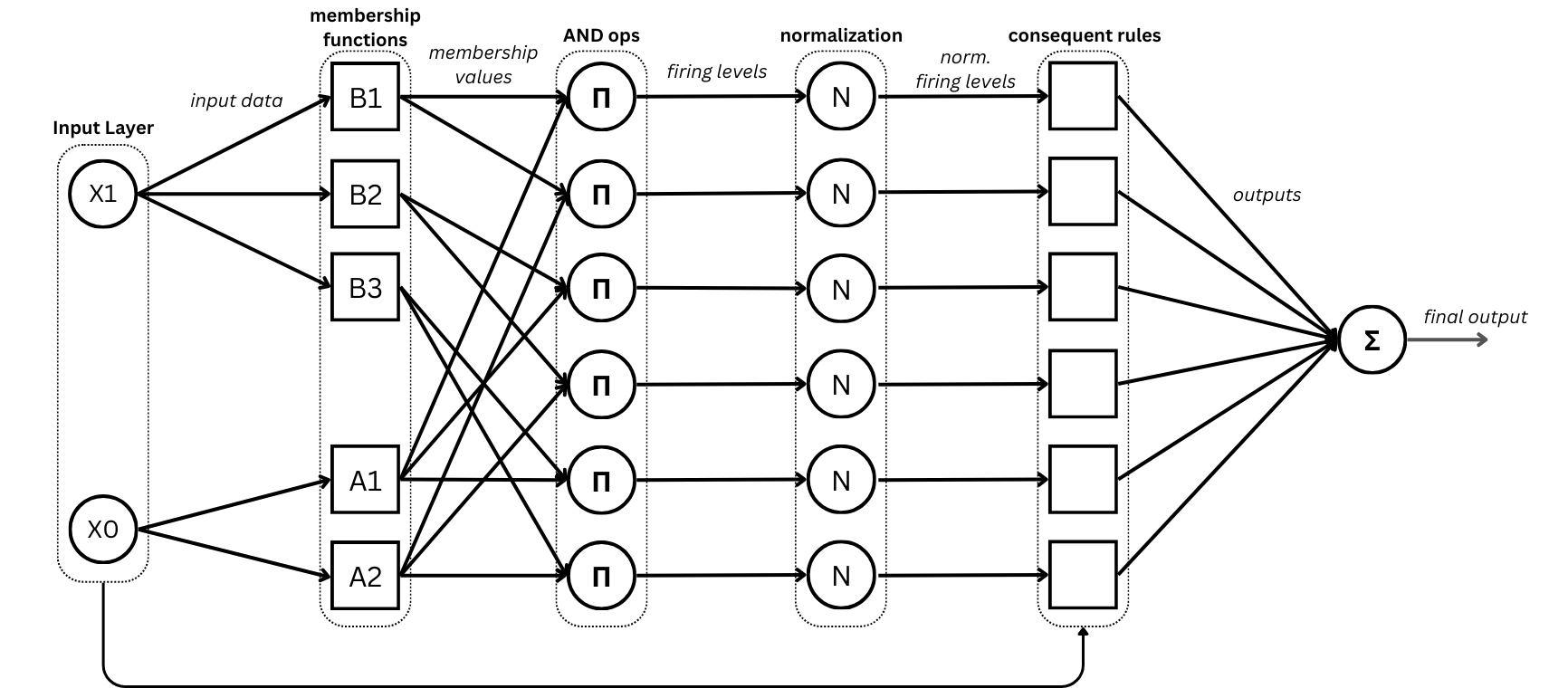
ANFIS model architecture (source: authors)

This section describes how to instantiate the classical ANFIS model implemented in Neuro-Fuzzy Toolbox and introduces some useful methods for interacting with it.

1. Import

import neuro_fuzzy_toolbox as nft
import torch

2. Instantiation

2.1 Instantiation parameters

The parameters available for instantiating an ANFIS model are the following:

• mf_distribution: List containing the number of membership functions for each input feature.

• outputs: Number of model outputs. Default is 1.

• membership_function: Membership function to use. Default is GeneralizedBell_MF.

• output_type: Defines the output layer of the model. Accepted values are 'default' (no output layer; classical mode for regression problems), 'sigmoid' (output layer with sigmoid activation), and 'softmax' (output layer with softmax activation). Default is 'default'.

• features: Iterable containing the names of the input variables considered by the model as strings. Default is None, which produces the list [x0, x1, …].

• dtype: Data type of the tensors holding the model parameters. Default is torch.float32.

2.2 Membership functions

The membership functions (MFs) available for the ANFIS model are the following:

Class Name	Membership Function
GeneralizedBell_MF	\(\frac{1}{1 + \left(\frac{|x - c|}{a}\right)^{2b}}\)
Gaussian_MF	\(e^{-\frac{(x - \mu)^2}{2\sigma^2}}\)
HighSlopeBell_MF	\(\frac{1}{1 + \left(\frac{|x - c|}{a}\right)^{2\cdot 8}}\)

Note

For more information on the membership functions implemented in Neuro-Fuzzy Toolbox, see API Reference - Membership Functions.

2.3 Instantiation example

The following example uses randomly generated data with 3 features.

# Simulating a dataset of 200 samples with 3 features
x_train = 2 * torch.rand(200, 3) - 1  # shape must be (200, 3)
y_train = torch.rand(200)              # shape must be (200,)

x_train

tensor([[ 0.9675,  0.4610,  0.3263],
        [-0.0157,  0.0160, -0.7043],
        [-0.8187, -0.3378,  0.4585],
        [ 0.2782, -0.5758,  0.7650],
        [-0.5861,  0.8199, -0.0063],
        ...

To instantiate an ANFIS model, the membership function distribution must first be defined according to the number of inputs (this is the only parameter with no default value and must therefore always be specified explicitly). This is done by providing a list containing the number of MFs for each input feature. For a 3-feature dataset, the following distribution can be defined:

mf_distribution = [3, 2, 3]

This specifies that the first and third features have 3 MFs each, while the second has 2.

The model can then be instantiated using the defined distribution:

model = nft.ANFIS(
    mf_distribution=mf_distribution,
    outputs=1,                               # 1 output
    membership_function=nft.GeneralizedBell_MF,
    output_type='default'
)

Note

All model parameters (premises and consequents) will be initialized randomly.

3. Selected Methods

The following methods are available for inspecting and interacting with an instantiated model.

Important

All methods presented in this section are valid for any ANFIS model variant implemented in Neuro-Fuzzy Toolbox. These variants are described in ANFIS Variants.

Premise visualization

The plot_premises() method plots the MFs of the model premises. Depending on the defined MF distribution, some subplots may be empty.

model.plot_premises()

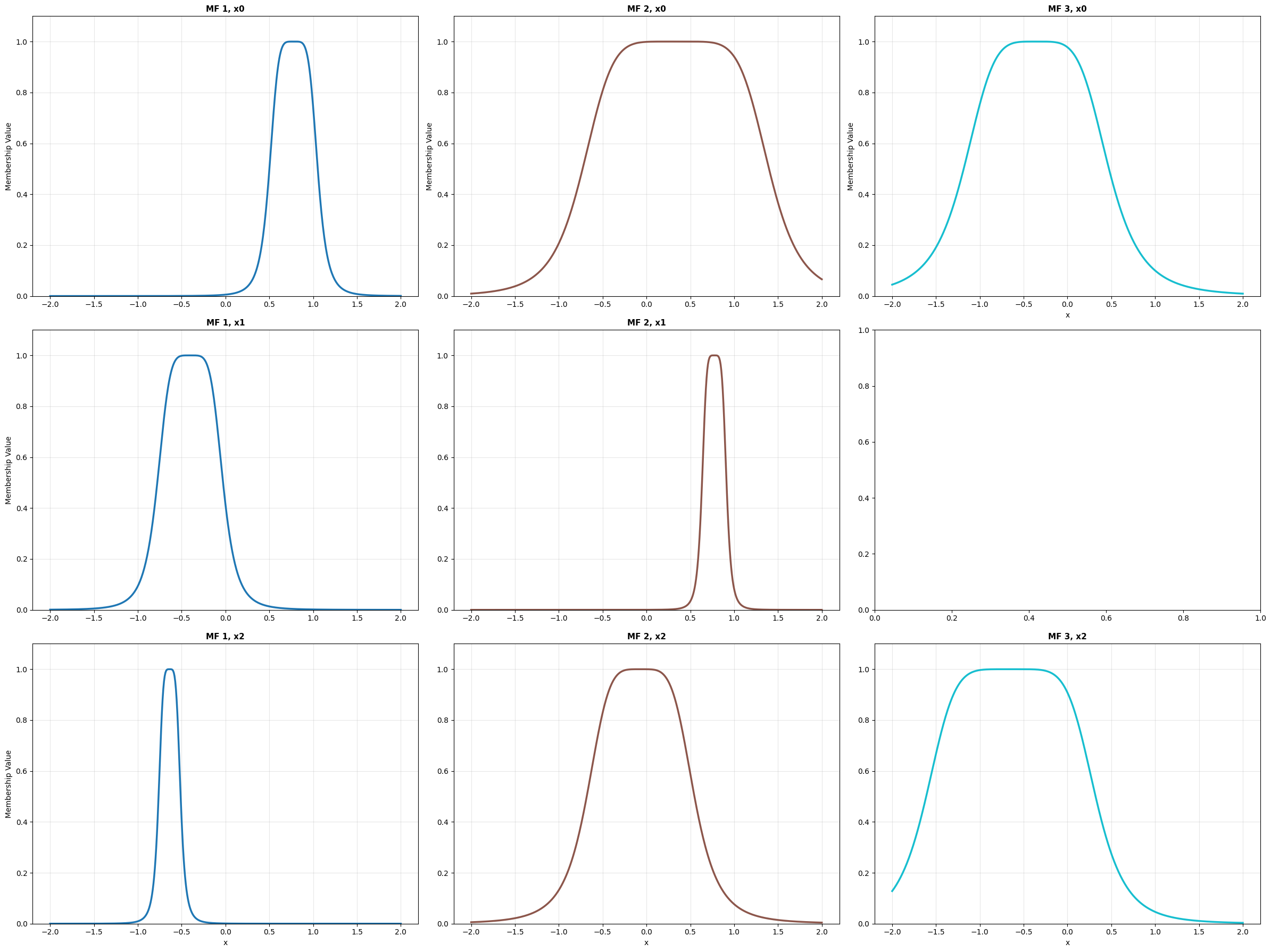
model.plot_premises() output

MFs can also be grouped by input dimension using the group_by_dim=True parameter.

model.plot_premises(group_by_dim=True)

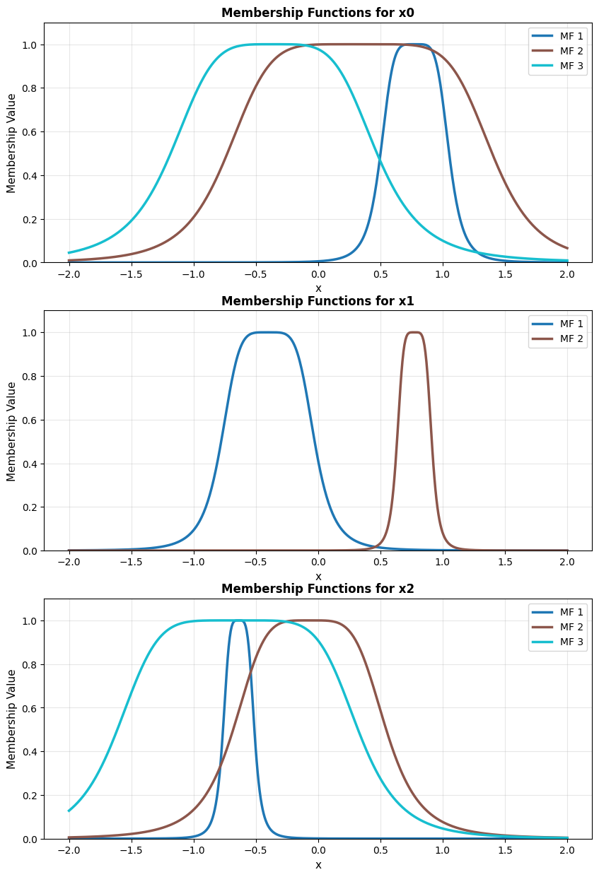
model.plot_premises(group_by_dim=True) output

Custom line styles that cycle across MFs can be specified via the linestyles parameter.

model.plot_premises(group_by_dim=True, linestyles=['-', '-.'])

model.plot_premises(group_by_dim=True, linestyles=[‘-’, ‘-.’]) output

Premise initialization

The init_premises() method initializes the premise parameters from the training data.

model.init_premises(x_train)

model.plot_premises(group_by_dim=True)

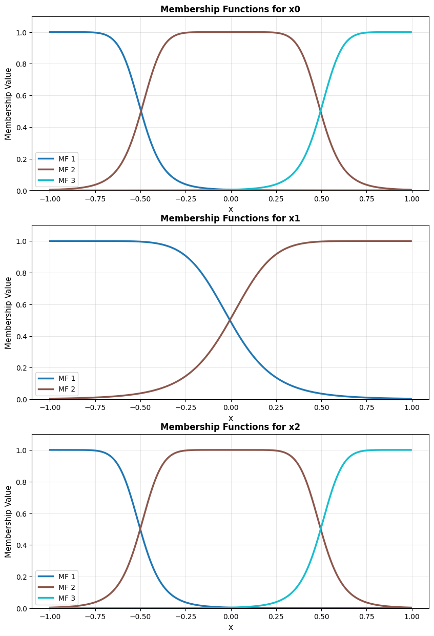
model.plot_premises(group_by_dim=True) output

Get premise values

The model.get_premises_structure() method returns the premise parameters in tabular form as a Pandas DataFrame (see Pandas Documentation).

df = model.get_premises_structure()
print(df.to_string())

            x0                            x1                            x2
             a         b         c         a         b         c         a         b         c
MF 1  0.275562  2.513212  0.776741  0.375067  2.445117 -0.402762  0.125963  2.208311 -0.637243
MF 2  1.063002  2.953724  0.334411  0.139761  2.501321  0.773252  0.614135  2.253394 -0.067316
MF 3  0.828421  2.231182 -0.355428       NaN       NaN       NaN  0.965939  2.838505 -0.645566

NaN values indicate that no MF exists for the corresponding feature at that position.

The model.get_premises() method returns the parameters in a more manipulation-friendly format: a list of tensors, one per input feature (of length input_size).

model.get_premises()

[tensor([[ 0.2756,  2.5132,  0.7767],
         [ 1.0630,  2.9537,  0.3344],
         [ 0.8284,  2.2312, -0.3554]]),
 tensor([[ 0.3751,  2.4451, -0.4028],
         [ 0.1398,  2.5013,  0.7733]]),
 tensor([[ 0.1260,  2.2083, -0.6372],
         [ 0.6141,  2.2534, -0.0673],
         [ 0.9659,  2.8385, -0.6456]])]

Note

In this case, each tensor has shape \((num\_mfs \times 3)\), where num_mfs is the number of MFs for that feature and 3 corresponds to the parameters \(a\), \(b\), and \(c\) of GeneralizedBell_MF. If Gaussian_MF were used instead, the shape would be \((num\_mfs \times 2)\), since Gaussian_MF has only two parameters (\(\mu\) and \(\sigma\)).

The model.get_premises_as_parameters_list() method returns the premises as an iterable of nn.Parameter objects stored internally in the model:

model.get_premises_as_parameters_list()

ParameterList(
    (0): Parameter containing: [torch.float32 of size 3x3]
    (1): Parameter containing: [torch.float32 of size 2x3]
    (2): Parameter containing: [torch.float32 of size 3x3]
)

To inspect the values:

for i, rule in enumerate(model.get_premises_as_parameters_list()):
    print(f"Feature {i+1} premises:\n", rule, "\n")

Feature 1 premises:
 Parameter containing:
tensor([[ 0.2756,  2.5132,  0.7767],
        [ 1.0630,  2.9537,  0.3344],
        [ 0.8284,  2.2312, -0.3554]], requires_grad=True)

Feature 2 premises:
 Parameter containing:
tensor([[ 0.3751,  2.4451, -0.4028],
        [ 0.1398,  2.5013,  0.7733]], requires_grad=True)

Feature 3 premises:
 Parameter containing:
tensor([[ 0.1260,  2.2083, -0.6372],
        [ 0.6141,  2.2534, -0.0673],
        [ 0.9659,  2.8385, -0.6456]], requires_grad=True)

Tip

The get_premises_as_parameters_list() method is useful for initializing PyTorch optimizers when implementing custom training procedures. See Custom training for details.

Get consequent values

Analogous methods are available for the consequent parameters. The model.get_consequents() method returns the consequent parameters stored in the model as a tensor of shape \((outputs \times num\_rules \times (input\_size + 1))\), where \(outputs\) is the number of model outputs, \(num\_rules\) is the number of rules, and \(input\_size + 1\) corresponds to the parameters of each rule (one coefficient per input feature plus the bias term).

model.get_consequents()

tensor([[[ 0.5301, -0.2289,  0.8846,  0.3022],
         [-0.4119,  0.3536,  0.1352, -0.3768],
         [-0.8613,  0.1430, -0.4151, -0.0445],
         [ 0.1645,  0.1320,  0.2322,  0.9766],
         [ 0.7077, -0.9880, -0.5299,  0.1812],
         [-0.6640,  0.8243,  0.2896,  0.6760],
         [-0.7384, -0.0971, -0.6692,  0.1911],
         [ 0.3822,  0.7965,  0.9330, -0.4947],
         [-0.9448,  0.8875, -0.0080, -0.5199],
         [-0.8340, -0.9991,  0.3486,  0.7330],
         [ 0.5894, -0.4916, -0.9528,  0.4650],
         [-0.0547,  0.2091,  0.7892,  0.2865],
         [ 0.4784, -0.4209,  0.9360,  0.7171],
         [-0.6172,  0.3039,  0.2237,  0.5542],
         [ 0.3943, -0.4589, -0.3258,  0.8626],
         [ 0.0125, -0.3117,  0.4590, -0.2067],
         [ 0.2149, -0.3138,  0.0204, -0.3937],
         [ 0.6653, -0.1333, -0.6162, -0.2090]]])

The model.get_consequents_structure() method returns the consequent parameters in tabular form as a list of Pandas DataFrames, one per model output.

dfs = model.get_consequents_structure()
for i, df in enumerate(dfs):
    print(f"Output {i+1}:\n", df.to_string(), "\n")

Output 1:
                x0        x1        x2
               c0        c1        c2        c3
rule 1  -0.382065  0.913401  0.874547  0.597923
rule 2  -0.089143  0.855073 -0.670351 -0.379125
rule 3   0.118713  0.616323 -0.208217 -0.854220
rule 4  -0.443418  0.714479  0.295737  0.059209
rule 5  -0.348620  0.352026 -0.341892  0.920784
rule 6  -0.675548 -0.300991 -0.240290  0.096369
rule 7  -0.665461 -0.537926  0.260524  0.317758
rule 8   0.973986  0.066278 -0.043222  0.356516
rule 9   0.048740 -0.179825 -0.103460  0.048633
rule 10  0.482887  0.163292 -0.209825  0.950138
rule 11 -0.155697 -0.112747 -0.608693 -0.597133
rule 12 -0.789493  0.679962 -0.805681  0.673177
rule 13  0.737387 -0.177445  0.334493  0.328383
rule 14 -0.557695  0.588001 -0.511353  0.470869
rule 15  0.770624  0.362488 -0.824404  0.275850
rule 16  0.562982  0.853030 -0.748265  0.331890
rule 17 -0.835750  0.076656  0.387303 -0.537785
rule 18  0.761043  0.821287  0.446539 -0.531705

The model.get_consequents_as_parameters_list() method returns an iterable of nn.Parameter objects holding the consequent parameters — in this case, stored as a single parameter:

model.get_consequents_as_parameters_list()

[Parameter containing:
 tensor([[[ 0.5301, -0.2289,  0.8846,  0.3022],
          [-0.4119,  0.3536,  0.1352, -0.3768],
          [-0.8613,  0.1430, -0.4151, -0.0445],
          [ 0.1645,  0.1320,  0.2322,  0.9766],
          [ 0.7077, -0.9880, -0.5299,  0.1812],
          [-0.6640,  0.8243,  0.2896,  0.6760],
          [-0.7384, -0.0971, -0.6692,  0.1911],
          [ 0.3822,  0.7965,  0.9330, -0.4947],
          [-0.9448,  0.8875, -0.0080, -0.5199],
          [-0.8340, -0.9991,  0.3486,  0.7330],
          [ 0.5894, -0.4916, -0.9528,  0.4650],
          [-0.0547,  0.2091,  0.7892,  0.2865],
          [ 0.4784, -0.4209,  0.9360,  0.7171],
          [-0.6172,  0.3039,  0.2237,  0.5542],
          [ 0.3943, -0.4589, -0.3258,  0.8626],
          [ 0.0125, -0.3117,  0.4590, -0.2067],
          [ 0.2149, -0.3138,  0.0204, -0.3937],
          [ 0.6653, -0.1333, -0.6162, -0.2090]]], requires_grad=True)]

Tip

Like get_premises_as_parameters_list(), the get_consequents_as_parameters_list() method is intended for initializing PyTorch optimizers and is used internally by the training algorithms implemented in Neuro-Fuzzy Toolbox. See Training for details on the available training algorithms and custom training procedures.

Consequent initialization

As with premises, consequents can also be initialized from data via a least-squares estimation:

model.init_consequents(x_train, y_train)

Note

For more information on this method and its implementation, see ANFIS API reference.

Get rule information

The classical ANFIS model generates fuzzy rules based on the combinatorial product of the MFs defined for each input feature. The model.rules property returns the total number of rules in the model.

model.rules  # In this case: 3 * 2 * 3 = 18

18

Detailed rule information can be retrieved with the model.get_rules_structure() method, which returns a Pandas DataFrame with the model parameters organized by rule.

df_rules = model.get_rules_structure()
print(df_rules.to_string())

         premises                                                                  output 1 consequents
               x0                       x1                       x2                                  x0        x1        x2
                a    b         c         a    b         c         a    b         c                   c0        c1        c2        c3
rule 1   0.485433  4.0 -0.998063  0.997669  4.0 -0.998142  0.497743  4.0 -0.999034             0.871878  0.826484  0.058868 -0.686231
rule 2   0.485433  4.0 -0.998063  0.997669  4.0 -0.998142  0.497743  4.0 -0.003548             0.174152  0.915871  0.700253 -0.695330
rule 3   0.485433  4.0 -0.998063  0.997669  4.0 -0.998142  0.497743  4.0  0.991938            -0.378210 -0.518292 -0.624950  0.475157
rule 4   0.485433  4.0 -0.998063  0.997669  4.0  0.997196  0.497743  4.0 -0.999034            -0.831691  0.423014 -0.144856  0.655579
rule 5   0.485433  4.0 -0.998063  0.997669  4.0  0.997196  0.497743  4.0 -0.003548             0.993477 -0.496301 -0.820423  0.251142
rule 6   0.485433  4.0 -0.998063  0.997669  4.0  0.997196  0.497743  4.0  0.991938            -0.323971  0.175129 -0.584292  0.300875
rule 7   0.485433  4.0 -0.027197  0.997669  4.0 -0.998142  0.497743  4.0 -0.999034            -0.775522  0.940813 -0.945905 -0.331948
rule 8   0.485433  4.0 -0.027197  0.997669  4.0 -0.998142  0.497743  4.0 -0.003548            -0.838004 -0.148445 -0.677109  0.593572
rule 9   0.485433  4.0 -0.027197  0.997669  4.0 -0.998142  0.497743  4.0  0.991938            -0.348051  0.568019  0.200678  0.959820
rule 10  0.485433  4.0 -0.027197  0.997669  4.0  0.997196  0.497743  4.0 -0.999034             0.862614 -0.960059  0.521483  0.946265
rule 11  0.485433  4.0 -0.027197  0.997669  4.0  0.997196  0.497743  4.0 -0.003548             0.110681  0.713140 -0.962105 -0.330632
rule 12  0.485433  4.0 -0.027197  0.997669  4.0  0.997196  0.497743  4.0  0.991938             0.660940 -0.452149  0.525000  0.271220
rule 13  0.485433  4.0  0.943669  0.997669  4.0 -0.998142  0.497743  4.0 -0.999034            -0.273925  0.425118  0.018813  0.599521
rule 14  0.485433  4.0  0.943669  0.997669  4.0 -0.998142  0.497743  4.0 -0.003548             0.224087 -0.539074 -0.348814 -0.732341
rule 15  0.485433  4.0  0.943669  0.997669  4.0 -0.998142  0.497743  4.0  0.991938            -0.748455 -0.223302 -0.001055  0.808488
rule 16  0.485433  4.0  0.943669  0.997669  4.0  0.997196  0.497743  4.0 -0.999034             0.803560 -0.220144  0.959322 -0.014778
rule 17  0.485433  4.0  0.943669  0.997669  4.0  0.997196  0.497743  4.0 -0.003548            -0.599493 -0.807238 -0.561908  0.364961
rule 18  0.485433  4.0  0.943669  0.997669  4.0  0.997196  0.497743  4.0  0.991938             0.787167  0.156500  0.121834 -0.989198

Note

For rule visualization and relevance evaluation methods, see Rule Inspection and Analysis.

4. Forward and predict methods

The forward method returns the model output for a batch of input data as a PyTorch tensor. This method constructs the PyTorch computational graph, enabling backpropagation and gradient-based training.

model(x_train[:10])

tensor([ 0.0515,  0.2146,  0.5617,  0.2492,  0.4197,  0.1205,  0.0435,  0.2851, 0.1256, -0.3293], grad_fn=<SqueezeBackward1>)

To suppress graph construction, use PyTorch’s no_grad context manager:

with torch.no_grad():
    output = model(x_train[:10])

print(output)

tensor([ 0.0515,  0.2146,  0.5617,  0.2492,  0.4197,  0.1205,  0.0435,  0.2851, 0.1256, -0.3293])

The predict method returns the model prediction for a batch of input data without constructing the computational graph. Depending on the output type, additional post-processing operations are applied to the result. Specifically, an argmax operation is used to obtain predicted class labels when the model has multiple outputs with a softmax output layer (see Output Types).

model.predict(x_train[:10])

tensor([ 0.0515,  0.2146,  0.5617,  0.2492,  0.4197,  0.1205,  0.0435,  0.2851, 0.1256, -0.3293])

Note

For information on the ANFIS model variants available in Neuro-Fuzzy Toolbox and their implications, see ANFIS Variants.